ICHEC Uses AI to Aid Disaster Recovery
ICHEC, Ireland's high-performance computing centre, recently participated in the xView2 disaster recovery challenge run by the US Defense Innovation Unit and other Humanitarian Assistance and Disaster Recovery (HADR) organisations. Models developed during the challenge including those developed at ICHEC are currently being tested by agencies responding to the ongoing bushfires in Australia.
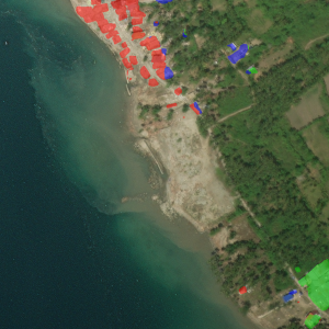
XView2 Challenge is based on using high resolution imagery to see the details of specific damage conditions in overhead imagery of a disaster area.
The challenge involved building AI models to locate and classify the severity of damage to buildings using pairs of pre and post disaster satellite images. Models like these allow those responding to disasters to rapidly assess the damage left in their wake, enabling more effective response efforts and potentially saving lives.
The challenge closed on the 31st of December, at which point ICHEC was ranked in the top 35 participants. In this post, Niall Moran, Senior Computational Scientist, describes ICHEC’s approach.
Challenge overview and difficulties
The competition organisers provided a dataset with pairs of high resolution satellite images and custom annotations for an area covering over 45,000 square kilometres, with over 850,000 annotated building polygons spanning six disaster types; floods, hurricanes, wildfires, earthquakes, volcanoes and tsunamis. A common standard called the Joint Damage Scale (JDS) was established for scoring the damage levels. Each building was assigned a level between between 0-3 corresponding to no-damage, minor-damage, major-damage and destroyed. Details of what these levels mean are shown in the table below.
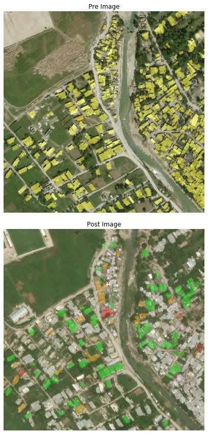
Some examples of the images with buildings and damage levels marked in for illustration.
A test-set of 933 image pairs were also provided for which there were no annotations. To compete in the challenge participants must submit their predictions on this test set, labelling which pixels are covered by buildings and the JDS damage level for each. From this, a score is calculated which is the weighted combination of scores for localising the buildings and classifying the damage levels. The damage classification score is weighted more highly with a weighting of 0.7 compared to 0.3 for the building localisation part. This leads to a balancing act as although the localisation score has a lower score weight it directly affects the score one can obtain in the damage phase.
The F1 score used is the harmonic mean of the per-pixel precision (proportion of true positives out of all positive predictions) and recall (proportion of true positives out of all true pixels). The F1 score while not as intuitive as measures like accuracy gives a much better indication of how well a model is working in the presence of unbalanced data. For example, in general the buildings cover a relatively small number of pixels. If we simply predict that all pixels are background, we can get an accuracy of 0.9 or higher even though our "model" has no predictive power. In this dataset there are also imbalances in the number of training samples from each disaster type, the distribution of disaster levels and the density of buildings in each image. To deal with these imbalances, we experimented with different loss functions including Dice [ref] and Focal losses [ref] which we describe below.
Our approach
Probably the most difficult and interesting aspect of the challenge is that it does not fit neatly into a standard problem class. This means there are no off the shelf models available offering an end to end solution. Tackling the problem necessitates combining multiple standard models and/or coming up with novel model architectures and objective functions, both of which require significant effort and experimentation. The problem that most closely matches is semantic segmentation where one attempts to label each pixel of an image according to the category it belongs to. This almost fits, but in this challenge we don't just have a single image for each case, but a pair of pre and post disaster images. The expected building footprints are based on the pre disaster images, whereas the damage level is based on the level of change between buildings in the pre and post disaster images.
The approach we followed in the time available was to split the problem into two separate parts which can be tackled with standard approaches - 1. identify the pixels with buildings in the pre disaster images and 2. classify the damage level of each of these by looking at the corresponding pixels in the post disaster images alone. By using the post disaster images alone for damage classification, we lose the context from the pre disaster images. Another issue with this type of approach is that because the damage classification phase depends on the building localisation, errors and inaccuracies are passed on and possibly made worse during the damage classification phase.
Building localisation
During our initial investigations we came across the [Solaris framework] (https://solaris.readthedocs.io/en/latest/) which is a machine learning framework developed specifically for geospatial imagery. It contains features for satellite imagery preprocessing and some pretrained models for building localisation. These models were from the [SpaceNet4](https://spacenet.ai/off-nadir-building-detection/) challenge which addressed building localisation from satellite imagery. We used the winning model from this challenge as a pretrained model as the basis for the localisation part of our pipeline. Starting with this pretrained model, we trained it some more with the xView2 training data to fine tune it and optimise it for the xView2 challenge dataset. The best model from this achieved an F1 score of 0.859 which wasn't far off the winning localisation score of 0.866. However due to the non trivial interplay between the building localisation output and the damage classification phase, we achieved a better overall score with a localization model that achieved the lower localisation score of 0.849.
Damage level classification
For the damage classification part of the challenge we used two different approaches.
First approach
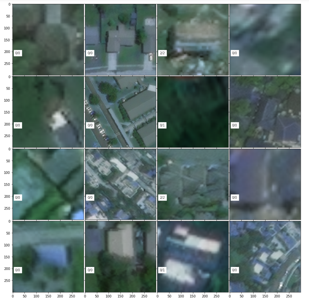
In the first of these we extracted image patches covering each annotated building from the post disaster images and using these trained a standard image classifier to predict the damage level of each building. To take into account the immediate surrounds of each building additional pixels around each building were included. The initial model used was a ResNet50 model initialised with pre-trained weights from the imagenet dataset. We then trained this model further using a weighted categorical cross entropy objective function. Next we experimented with combined objective functions with components of Dice loss, Focal loss and categorical cross entropy, training with different patch sizes (300x300 and 224x224 pixels), and using the ResNext101 model architecture as a backbone network. With ensembles of these models, we reached a damage F1 score of 0.64. The figure below shows an example of what the image patches for buildings look like.
Second approach
For the second approach we used semantic segmentation models to predict the damage level of each pixel of the post disaster image. The objective function used was a weighted multi-class focal loss function. The weight for each damage level was set so that it is proportional to the inverse frequency of the occurrence of the level. This resulted in the minor-damage and major-damage levels being weighted highest, followed by the destroyed level and finally the no-damage level with the smallest weight. The background pixels were weighted zero so they were effectively ignored. This allowed the model to create large regions around buildings with the same damage level. We think this is particularly effective for this problem as in the majority of disasters the same level of damage generally affects groups of buildings in the same region. The following figure shows some images where this is apparent.
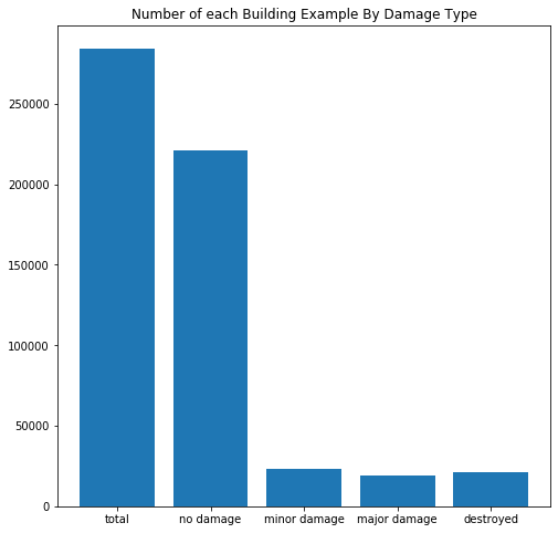
Figure showing the imbalance of damage types for training the damage assessment network.
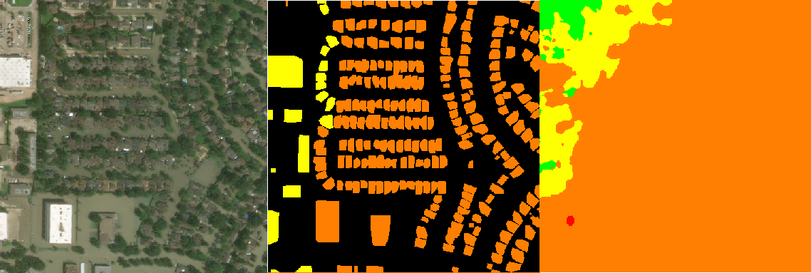
Figure showing post disaster image, the ground truth damage levels for each building and the predicted damage levels.
We experimented with a number of different model architectures, image sizes and hyper parameters for this model. The best damage score we got was just short of 0.71. This was using an ensemble of the six best models (from local validation). The ensemble consisted of 3 pairs of models trained on 512x512 images. The model architectures were Encoder Decoder models with DenseNet121 and DenseNet161 backbones and a UNet model with a ResNet34 backbone. This together with a localisation model that scored 0.849 gave us an overall score of 0.752 putting us in 32nd place. The top score was 0.805 (0.778 damage and 0.866 localisation) and the cut-off for the top 50 leaderboard was 0.718 (0.651 damage ad 0.875 localisation) so there wasn’t a huge spread.
Conclusions
During this challenge we found ourselves pulled in many different directions. It’s always difficult to know when to stick to established methods and try to eke out any remaining performance gains from things like tuning the hyper parameters, training for longer or to try something new and unproven with the risk that it may struggle to even reach the performance that’s already been achieved.
Over the course of the challenge we tried a number of things which didn’t give the improvement we expected. This could have been that they were bad ideas, errors in our implementation or just that we were missing some additional consideration required to make them work. Somethings we tried were stacking pre and post images so that the input had six channels, using the difference between pre and post images as input and using a loss function that takes into account the ordinal nature of the damage levels.
Some approaches and techniques we found that worked well that we made good use of and could potentially have prioritised more:
Using ensembles of different models with different architectures and trained using different splits of the training data. This reliably provided an improvement in performance which can be attributed to the strengths of the different models complementing each other.
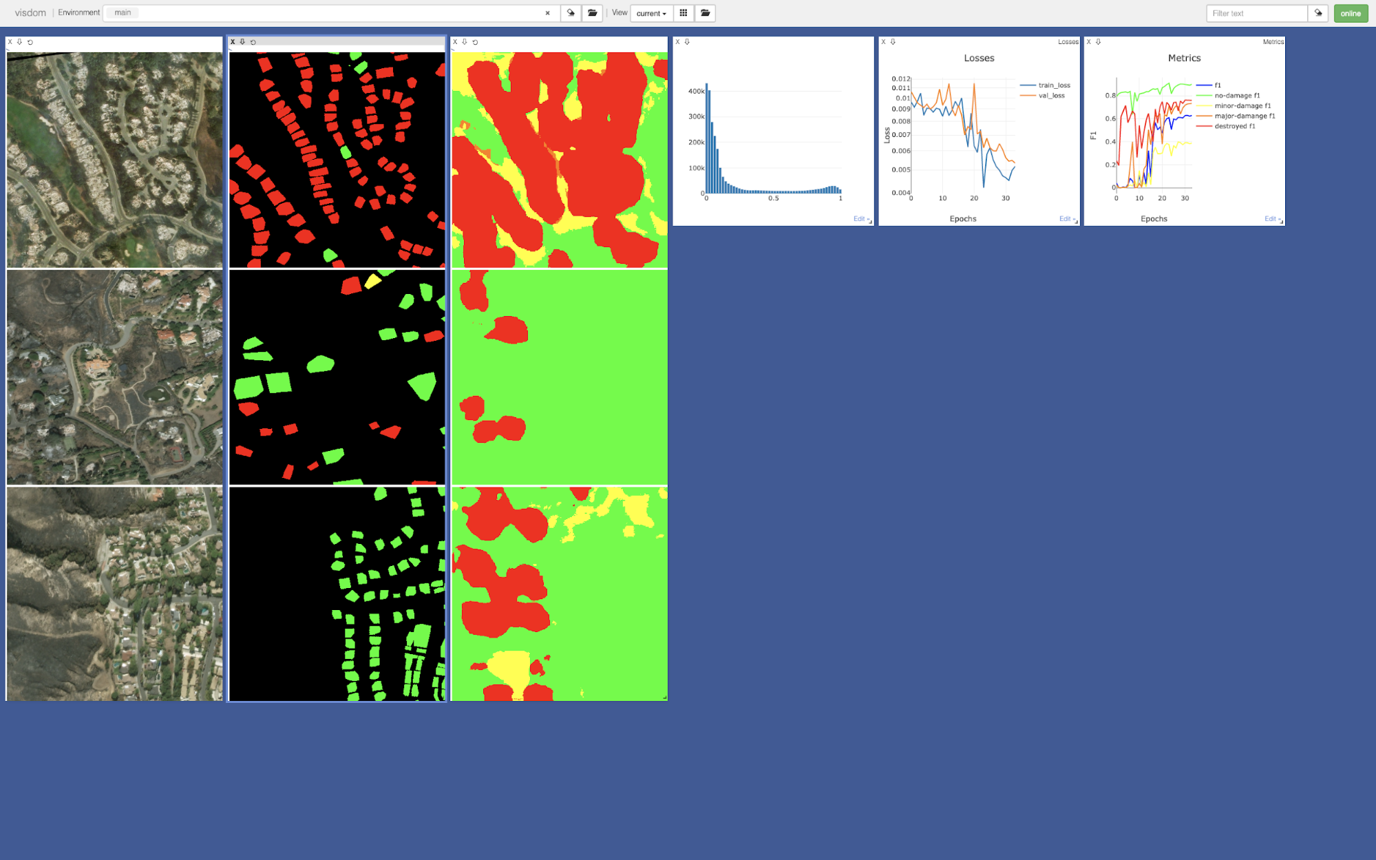
Spending time on creating visualisations to get a better understanding of the data and what the models are doing and find mistakes early. For this we used [fast.ai](https://www.fast.ai/) callbacks and [Visdom](https://github.com/facebookresearch/visdom) which makes it very easy to create interactive dashboards.
Taking the time, particularly early on in the challenge to clean up code and align with others on the team. This can be difficult in challenges like this where there are always new things to add and try.
Screenshot of the visdom dashboard we developed to monitor training our damage models. Indicates how the model is working.
We look forward to applying these to earth observation projects at ICHEC and in future challenges.
One such challenge is the SpaceNet6 challenge which starts in March and involves Synthetic Aperture Radar (SAR) images. These images can be taken at night and are not obscured by clouds, something that is particularly relevant in the Irish context, where we have some of the highest rates of cloud cover in the world.